Category: Power Query

Power Query Free Training Webinar Follow-Up Questions

On April 7th, I gave my Power Query: Data Chemistry for the Masses presentation as part of Pragmatic Works Free Training on the T’s series. You can find the recording of that webinar here. I want to take a moment to thank the folks at Pragmatic Works for organizing and hosting this series that is such a great asset to the community.

At the end of the session, there were more questions than we had time to handle. So, they emailed me the questions in order for me to answer them in a post like this. Behold!

What is the maximum number of rows allowed in an Excel worksheet?

This question was likely in response to my recommendation of loading Power Query results to the Excel Data Model (Power Pivot) instead of to a worksheet. According to this info from Microsoft, the maximum row count in a worksheet is 1,048,576.

When combining files in a folder can the workbook have multiple tabs?

As far as combining files using the From Folder source, I have only succeeded with text files. However, there is a post here on the Dutch Data Dude blog that explains how to combine that source with a little custom M to make this happen.

When passing a parameter to an M function, can you select from a pick list of choices?

This question was in response to my converting a power query on Nobel Prize Laureates into a function that prompts for a prize category and then returns the Laureates for that category. Typically, instead of users interacting directly with the function, the parameter is passed to the function via a custom column. There is great post here on the Data Chix blog on how to do this.

Could we get a copy of the file being used in the demo?

You can get all of the materials for the presentation, including the files used, on the page for that presentation on this very blog.

Is the option to load to data model available for Excel 2010 or later versions?

I just learned over the weekend at SQL Saturday Madison that Excel 2010 does NOT have the option to load directly to the Data Model. Bummer. So, if you are using Excel 2010, you will need to load to a worksheet and then import to Power Pivot from that worksheet.

How do you know a web page is in JSON?

Well, web pages are not really in JSON. JSON is actually a “lightweight document interchange format.” I think of it more like a simpler XML. This question comes from my use of the Nobel Prize API to download Laureate data in the JSON format as part of this presentation. This is also detailed here as part of my Power Query Decathlon – Beginner blog series. The URL for consuming the API using JSON is http://api.nobelprize.org/v1/laureate.json. You can also do it as a CSV using http://api.nobelprize.org/v1/laureate.csv which will actively download a CSV file with all of the same data.

What do the different separators mean? [] i guess means column, but what is {} for?

I assume this question is related to the appearance of [] and {} in M query syntax. You can read about these in the Query Formula Language Specification document. This is a large resource and not recommended for “light” reading. 🙂 According to the specification, “We can use the lookup operator ([]) to access the fields of a record by name.” Also, the brackets [] can be used for referring to Records by surrounding the elements within the Record. the {} curly braces are used to referring to a List. A great, and easy to follow, resource is Chris Webb’s great book Power Query for Power BI and Excel. I am still very much a student of M, so I will not go much deeper into this at the moment.

Any plan from MS to add the ability to export the resulting data to a place other than XL, Data Model, eg text file, db?

I would LOVE the ability to use Power Query to load data into a database or a file, etc. Note that Power Query is used outside of Excel for loading data in the new Power BI preview as well as the Power BI Designer, which is also currently in preview. I have yet to see public information regarding any detailed plans for using Power Query to load to a larger number of targets. However, given the investment Microsoft is making in Power Query, it seems likely to me that we will see it popping up in more places in the future.

Could we use an Itunes folder as a source and consolidate music metadata?

Yup.

Here is the M code for a query I used to do just that:

let
    Source = Folder.Files("C:\Users\Mark\Music\iTunes\iTunes Media\Music"),
    #"Removed Other Columns" = Table.SelectColumns(Source,{"Name", "Folder Path"}),
    #"Replaced Value" = Table.ReplaceValue(#"Removed Other Columns","C:\Users\Mark\Music\iTunes\iTunes Media\Music\","",Replacer.ReplaceText,{"Folder Path"}),
    #"Split Column by Delimiter" = Table.SplitColumn(#"Replaced Value","Folder Path",Splitter.SplitTextByEachDelimiter({"\"}, null, false),{"Folder Path.1", "Folder Path.2"}),
    #"Changed Type" = Table.TransformColumnTypes(#"Split Column by Delimiter",{{"Folder Path.1", type text}, {"Folder Path.2", type text}}),
    #"Replaced Value1" = Table.ReplaceValue(#"Changed Type","\","",Replacer.ReplaceText,{"Folder Path.2"}),
    #"Split Column by Position" = Table.SplitColumn(#"Replaced Value1","Name",Splitter.SplitTextByPositions({0, 2}, false),{"Name.1", "Name.2"}),
    #"Changed Type1" = Table.TransformColumnTypes(#"Split Column by Position",{{"Name.1", Int64.Type}, {"Name.2", type text}}),
    #"Split Column by Delimiter1" = Table.SplitColumn(#"Changed Type1","Name.2",Splitter.SplitTextByEachDelimiter({"."}, null, false),{"Name.2.1", "Name.2.2"}),
    #"Changed Type2" = Table.TransformColumnTypes(#"Split Column by Delimiter1",{{"Name.2.1", type text}, {"Name.2.2", type text}}),
    #"Renamed Columns" = Table.RenameColumns(#"Changed Type2",{{"Name.1", "Track"}, {"Name.2.1", "Song"}, {"Name.2.2", "File Type"}, {"Folder Path.1", "Artist"}, {"Folder Path.2", "Album"}})
in
    #"Renamed Columns"

In the Code above, I highlighted the path to my Itunes folder. Just replace that with yours and past into a blank Power Query window. Here is the query once you have done so.

image

There is more data in the Itunes Music Library.xml file, but I haven’t figured out how to use it effectively yet.

Alright. That wraps up the questions. Thanks to all who tuned in to the webinar and provided such great questions.

Advanced Column Splitting in Power Query

A friend of mine left a question on one of my Power Query Decathlon posts asking if it was possible to split a column using a carriage return as a delimiter. After a little poking around myself, I was not finding the answer I sought. So, I reached out for help. Curt Hagenlocher, a developer at Microsoft was kind enough to help me out. As it turns out, it appears that splitting a column based on carriage returns does not work. However, you CAN split columns based on the line feed character.

Note: M is actually informal name for the Power Query Formula Language.

The sample data

First, I created a collection of lines of text separated by using the <Enter> key. I did this in NotePad++, a free but powerful utility. I activated the feature which allows viewing of all non-printing characters. That is shown in Figure 1.

Figure 1

image

In Figure 1, you can clearly see the CR and LF characters after lines 1 and 2.

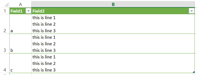
I then highlighted this block of text and pasted it into each of the cells in Field2 in the table in Excel shown in Figure 2. Not, I had to paste this into each cell using the formula bar, not into the cells directly.

Figure 2

image

The result is a very simple table where all of the values in Field2 contain <CR><LF> characters, hidden by default.

I then added a query with this table as its source by using the From Table button on the Power Query Ribbon. The result is the query shown in Figure 3.

Figure 3

image

This is our starting point for two different solutions.

M-less Solution

The first, and easiest solution starts with a simple Split Column transformation on the Field2 column. Figure 4 shows how to configure the Split Column for this example.

Figure 4

image

We start by creating a basic Split Column making sure of the following:

  1. Select whichever delimiter you want. However, it is best if you can find one that actually does not appear in the data.
  2. Make sure the “At each occurrence of the delimiter” option is selected. This is the default, anyway.
  3. Since there are a total of 3 lines of text in our Field2 domain of values, we need to set the “Number of columns to split into” option. You would think that the option indicating to split on each delimiter would mean this step would not be necessary. Unfortunately, as least as of the March 2015 update of Power Query, it is.

When you click OK, the result is shown in Figure 5.

Figure 5

image

Since there are no commas in this text, the result is a total of three columns, but only one of them has data. However, this is a necessary first step. The use of non-printing characters as delimiters is not supported by the Power Query UI. So, we need to manually edit the M for the Split Column by Delimiter step. Yes, I know I said this was M-less. However, the edit that is required is tiny and you are not really writing any M.

Figure 6 shows the unmodified M code for the Split Column by Delimiter step.

Figure 6

image

Notice the delimiter shown by the arrow. It is the comma since that is what we chose for this step initially. In order to change that to the <LF> character, we replace that comma with the #(lf) value as show in Figure 7.

Figure 7

image

The result of this change is shown in Figure 8.

Figure 8

image

Great, right? Awesome? Well, sort of. While this worked in our very simple situation in which we knew how many line of text were present, this was OK. And if that is your situation, then hazzah! However, reality is typically more complicated than that.

I saved this query as M-less in the Excel file provided with this post.

M-ful Solution

The more elegant and flexible solution requires M. And, I am still very much a student of M, and a beginner at that. The M code featured in this solution was provided by Microsoft’s Curt Hagenlocher, mentioned above, who was tremendously helpful in answering this question and very patient with my M noobness.

With this solution, the first step after the source is to change the data type of Field2 to Text. While I tried it without this step and it worked just fine on my simple sample data, it is not a bad precaution to ensure the Field2 column is text before proceeding. So, I left it in. The result is shown in Figure 9. Note that this is the last step in this solution that can be accomplished in the UI. It is all M from here.

Figure 9

image

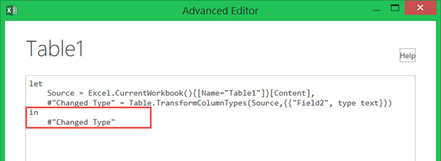
There isn’t much to see here. But if you click on the View tab of the ribbon and then click on the Advanced Editor, you will see the M code for the entire query. That is shown in Figure 10.

Figure 10

image

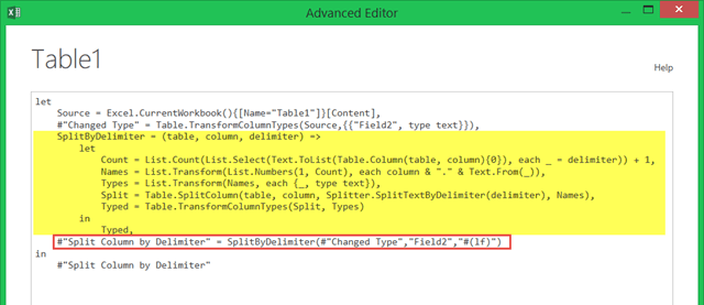
The next step is to paste in the M provided by Curt. That code replaces the bottom section of the query, shown in the rectangle. Once the new code is pasted in, we will highlight a few parts. The final query is shown in Figure 11.

Figure 11

image

The entire query is pasted below to make it easy for you to copy. Note that, following the pattern of how M works, each step in the function, shown highlighted, has a name that is then referenced by subsequent steps.


let
    Source = Excel.CurrentWorkbook(){[Name="Table1"]}[Content],
    #"Changed Type" = Table.TransformColumnTypes(Source,{{"Field2", type text}}),
    SplitByDelimiter = (table, column, delimiter) =>
        let
            Count = List.Count(List.Select(Text.ToList(Table.Column(table, column){0}), each _ = delimiter)) + 1,
            Names = List.Transform(List.Numbers(1, Count), each column & "." & Text.From(_)),
            Types = List.Transform(Names, each {_, type text}),
            Split = Table.SplitColumn(table, column, Splitter.SplitTextByDelimiter(delimiter), Names),
            Typed = Table.TransformColumnTypes(Split, Types)
        in
            Typed,

    #"Split Column by Delimiter" = SplitByDelimiter(#"Changed Type","Field2","#(lf)")
in
    #"Split Column by Delimiter"


The steps in the function, as clearly as I can understand/explain them, are as follows:

Count = This step takes in the parameters for the table and the column and examines the contents in the column to discover how many times the delimiter passed in the parameter occurs in that column. This allows the function to dynamically create the correct number of columns instead of having to hard code it like we had to do in the M-less Solution.

Name = This step creates column names for as many columns as were determined in the Count step. The name for each column is prefaced with the original column name passed into the function.

Types = This step creates a list object containing all of the column names created by the Name step and appends to each the code necessary to converting them to text. This column will be used in a subsequent step to make it easy to convert all of the columns to text before exiting the function. This is cool. 🙂

Split = This step uses the Splitter.SplitTextByDelimiter function to perform the splits of the column into the columns provided in the Name step above using the specified delimiter.

Typed = This step uses the list of column names and the strings from the Types step to convert all of the newly created columns to Text. The results of this step are then returned from the function.

That completes the function walkthrough. Pretty neat, if you ask me.

The final step of the query is to invoke this function. This is done via the section of code in the red rectangle in Figure 11. For the table parameter of the function, this step uses the Changed Type query step we performed in the UI. This is a great example of how steps in queries, at least in M, are not limited to referencing only the single step that immediately preceded them.

The final result is shown in Figure 12.

Figure 12

image

This query was saved a M-ful in the working file provided.

NOTE: Neither of these solutions work for the <CR> character. So, replacing the #(lf) above for #(cr) does not produce the desired result. I even tried using #(cr)#(lf) and that does not work either. Just #(lf) worked for me.

There you have it. You can find the working file I used for this post right here.

One of the aspects I like best about blogging is the learning I get out of it. In order to try to explain things clearly in my posts, I need to study them and understand them. Through a previous post, I got a great question I had not thought about. Through the investigation, I found yet another great and helpful person within Microsoft in Curt Hagenlocher. In putting this post together, I obtained a far greater understanding of M and it capabilities than I had before.

Power Query Decathlon – Beginner 10: Query Management

NOTE: This post was created using the November 2014 version of Power Query. In later versions, some of the screens or functionality could be different.

You can download the Excel 2013 file necessary to perform the steps in this post here. To get to the existing query, click the Workbook Queries button on the Power Query ribbon.

For the final post in this series, we cover Query Management. There are several options available. We begin with our Workbook Queries pane.

1. Right-click the Laureate query to reveal the menu shown in Figure 1.

Figure 1

image

The query management options on this menu are as follows:

  • Edit – This allows you to open the query in the Query Editor
  • Delete – um…. this lets you delete the query. Note: If you delete the query, any tables loaded from this query will also be deleted.
  • Refresh – This will execute this query, loading fresh data to the configured Load destination. The Laureate query in Figure 1 is set to Loan nowhere, so the Refresh button is grayed out.
  • Load To – This option lets you change the destination to which this query loads.
  • Duplicate – This makes a full duplicate of this query including the source and all the steps.
  • Reference – This lets you make a new query that uses this query as its source.
  • Merge – This lets you create a new query that combines columns from this query with another.
  • Append – This lets you create a new query to adds the rows from a second query onto this one, rather like a UNION in T-SQL.
  • Send To Data Catalog – This allows you to save this query into the Power BI Data Catalog so you can share it with other Power BI users.
  • Move To Group – This lets you create folders within the Workbook Queries pane to organize your queries.
  • Move Up/Down – This lets you alter the position the query occupies in the Workbook Queries list.
  • Show the Peek – This allows you to bring up the Peek (preview) pane for this query.
  • Properties – This allows you to change the Name and/or Description for this query.

We will not cover all of these in this post. We will just do a few of them. The options we will cover are Reference, Merge, and Append.

Reference

To have one query use another query as its source, we use Reference.

2. From the menu in Figure 1, choose the Reference option, as shown in Figure 2.

Figure 2

image

This will create and execute a new query, using the selected query as its Source and using the default Load options. The result should resemble Figure 3.

Figure 3

image

The new query takes the name of the first query with an ordinal added. Figure 4 shows the Power Pivot table that was created as a result.

Figure 4

image

I just wanted to show this to make you aware that you may need to change names in your data model manually when you use this technique.

3. Double-click the Laureate (2) query to open it in the Query Editor, as shown in Figure 5.

Figure 5

image

You can see that the Source for the query is Laureate, not the Nobel Prize api that we originally used.

We will modify Laureate (2) to return only the Individuals (not organizations) that won prizes and name it accordingly.

4. Click the filter button in the Gender query header.

5. Click the Org option to deselect it, as shown in Figure 6.

Figure 6

image

6. Change the name of the query, in the PROPERTIES box to Individual Laureates, as shown in Figure 7.

Figure 7

image

7. Use Ctrl-Click to select both the Award Year and Award Category columns, as shown in
Figure 8.

Figure 8

image

8. Click the Group By button, shown by the arrow in Figure 8. This will launch the Group By dialog shown in Figure 9.

Figure 9

image

9. Click OK. The results should resemble Figure 10.

Figure 10

image

10. Click the Close & Load to save this query. This will save the changes to this query and execute it. The Workbook Queries pane should now resemble Figure 11.

Figure 11

image

We now have a summarized count of Individual Laureates by Award Year and Award Category.

Note: When I first started playing with Reference, I thought it would be a way to break a single source into multiple tables and minimize the impact on the source by only hitting that source once. My testing has shown me that that is not how it works. In the example above, executing (Refreshing) the Individual Laureates query will actually just include all the steps from the Laureate query when it runs. So, rather than execute the Laureate query and then use those results as a source, Power Query takes the steps from the Laureate query and includes them when executing any query Referencing the Laureate query. I tested this by creating a single query against a SQL Server table. I then created 4 other queries via the Reference method above. Tracing the SQL Server instance confirmed that the query was actually querying the source for each and every query, not just once. It seems to me, though, that there could be some advantage if you need to use the same source table multiple times and only want to build the steps to clean up that table once. So, in that sense, the Reference method could be a way to modularize your steps so you can maintain them in one place.

11. Create another Reference query based on Laureate. This will create Laureate (2) again.

12. Edit that query to return ONLY the Org values from the Gender column, as shown in Figure 12.

Figure 12

image

13. Give the query an appropriate name like Organization Laureates, as in Figure 13.

Figure 13

image

14. Use Ctrl-Click to select both the Award Year and Award Category columns, as shown in
Figure 14.

Figure 14

image

15. Click the Group By button, shown by the arrow in Figure 14. This will launch the Group By dialog shown in Figure 15.

Figure 15

image

16. Click OK. The results should resemble Figure 16.

Figure 16

image

17. Click the Close & Load to save this query. This will save the changes to this query and execute it. The Workbook Queries pane should now resemble Figure 17.

Figure 17

image

Note: When a Reference is made to a query by another, Laureate in this case, any changes to the referenced query can break the queries that reference it. So, in our example, making changes to Laureate could cause the other queries to become invalid. Just bear that in mind when deciding to use Reference.

Merge

Merge allows you to combine columns from one query into another, rather like joining tables together in a SQL query.

18. Right-click on the Individual Laureates query to reveal the menu shown in Figure 18.

Figure 18

image

19. Click the Merge option to launch the Merge dialog shown in Figure 19.

Figure 19

image

The query we chose, Individual Laureates, appears in the top section. This will be out main table. In the bottom section, we will choose the table from which to add columns to Individual Laureates.

20. Click the drop-down shown by the arrow in Figure 19. This will allow us to select the marge table, as shown in Figure 20.

Figure 20

image

21. Choose Organization Laureates. The dialog should now resemble Figure 21.

Figure 21

image

This is where we tell Power Query which columns to use for merging the tables so that rows in Individual Laureates can find matching rows in Organization Laureates.

22. Click the Award Year column heading under the Individual Laureates query, shown by the 1 in Figure 21.

23. Click the Award Year column heading under the Organization Laureates query, shown by the 2 in Figure 21. The dialog should now resemble Figure 22.

Figure 22

image

Note: It is not strictly necessary to always choose the column from the top query first. I just find it more intuitive. You can choose the Award Year column from Organization Laureates and THEN the one from Individual Laureates and this will still work just fine.

Once at least one join column has been specified for both queries, Power Query will indicate how many rows from the lookup query (Organization Laureates in this case) match rows in the main query. The highlighted message at the bottom of Figure 22 indicates that 110 or the 550 rows in Individual Laureates found matching rows in Organization Laureates when joining on Award Year.

For our merge example, we will join not just on Award Year, but on Award Category as well. I realize this is a pretty silly join since it will only match on rows where a specific award was shared by at least one Individual and an Organization. But, the mechanics of joining on more than one column are important.

24. Ctrl-Click the Award Category column heading under the Individual Laureates query, shown by the 1 in Figure 22. You must use Ctrl-Click so that Power Query knows that you are specifying an additional join column and not changing the join column selection you initially made.

25. Ctrl-Click the Award Category column heading under the Organization Laureates query, shown by the 2 in Figure 22. The dialog should now resemble Figure 23.

Figure 23

image

Here we can see both join columns selected in both queries. Since it is hard to see in Figure 23, Figure 24 shows a closer view of the column headings for the merge.

Figure 24

image

The 1 in the Award Year column header and the 2 in the Award Category column header indicate that we are joining first on Award Year and then on Award Category.

26. Click OK. The query should resemble Figure 25.

Figure 25

image

Our next step is to rename the Count column for the Individual Laureates query, shown by the arrow in Figure 25. The reason is that both queries contain a column named Count and and we cannot have duplicate columns names in a single query. Beside, Count is a pretty terrible name anyway. 🙂

27. Double-click the Count column header. It was pointed out to me in a comment on a previous post that I did not mention this method for renaming columns. Therefore, we shall use it here.

28. Give it a meaningful name like “Individual Count.” The query should now resemble Figure 26.

Figure 26

image

29. Click the Expand button, shown by the arrow in Figure 26. This will reveal the columns available from the Organization Query, as shown in Figure 27.

Figure 27

image

30. Change the selection so that only the Count column is selected, as in Figure 28.

Figure 28

image

Note the “Use original column name as prefix” checkbox. With this checked, the default, the new columns pulled from this query will be prefaced with “NewColumn” since that is the name of the merged column. I typically turn that off but will leave it on here in order to show what that looks like.

31. Click OK. The query should resemble Figure 29.

Figure 29

image

32. Rename the NewColumn.Count column to something more appropriate like “Organization Count.”

33. Change the name of the query in the PROPERTIES area to Merge Example. The query should not resemble Figure 30.

Figure 30

image

34. Close & Load. The Workbook Query pane should now resemble Figure 31.

Figure 31

image


Note: The Merge option is available when you editing an existing query. In that case, it will bring the new columns into THAT query instead of creating a brand new query that is the end result of the merging.

Append

The Append option allows you to basically stack all the rows from one query underneath the rows of another query. The result is a single query with all of the rows from both. It is important that the queries to be merged have the same structure.

35. Right-click the Individual Laureates query to bring up the menu shown in Figure 32.

Figure 32

image

36. Choose Append, shown by the arrow in Figure 32. This will bring up the Append dialog shown in Figure 33.

Figure 33

image

37. Use the drop-down shown by the arrow in Figure 33 to select Organization Laureates as the one to append. The dialog should now resemble Figure 34.

Figure 34

image

38. Click OK. The query should resemble Figure 35.

Figure 35

image

39. Name the query Append Example.

40. Close & Load. The Workbook Queries pane should now resemble Figure 36.

Figure 36

image

The Append Example query has 573 rows (550 from Individual Laureates and 23 from Organization Laureates).

Note: You can use the Append option when you are editing an existing query. In that case, the rows from the second table will be appended to the rows in THAT query instead of creating a new query.

Conclusion

That brings this Power Query Decathlon – Beginner series to an end. I hope you found it helpful and that you see what an exciting tool Power Query is.

Power Query Decathlon – Beginner 09: Loading Results

NOTE: This post was created using the November 2014 version of Power Query. In later versions, some of the screens or functionality could be different.

You can download the Excel 2013 file necessary to perform the steps in this post here. To get to the existing query, click the Workbook Queries button on the Power Query ribbon.

Once you have constructed your query, it is time to Close & Load it. This is the process of saving the query for use and also, optionally, executing it at the same time.

You have a total of 4 options for loading your query results:

  • Load it to the Excel Data Model (Power Pivot) in the same Excel workbook housing the query (This is the option I use most frequently and recommend highly)
  • Load it to a worksheet in the same Excel workbook housing the query (the Default)
  • Load it to the Excel Data Model AND a worksheet
  • Load it to neither of the above options (load it nowhere at all, just creating the query)

Note: Up to this point, I have kept the default name for the query we have used, Query1. I have closed and loaded it several times with this name. However, I advise you, with your own queries, to give them appropriate names before you Close & Load them. I just wanted to keep the focus of each post narrow and didn’t want to deal with it until now.

Load to Data Model

We will start this post by opening our existing query and giving it a proper name.

1. Double-click the query Query1 you see in the Workbook Queries pane of the Power Query ribbon, as shown in Figure 1.

Figure 1

image

This will open the Query Editor shown in Figure 2.

Figure 2

image

The name of the query is found in the PROPERTIES section of the Query Settings pane, just above the APPLIED STEPS. The query name will determine the name of the table when the data is loaded. For example, so far, I have been loading my query to the Data Model. So, if I open my Power Pivot management window in this file, we can see there is a single table there called Query1, as shown in Figure 3.

Note: I am not expecting you to take this particular step. I show this merely for illustration.

Figure 3

image

This is the final destination for the data that runs through the Query1 query.

2. Give your query an appropriate name in the PROPERTIES, such as Laureate. An example is shown in Figure 4.

Figure 4

image

3. Click the Close & Load button, shown by the arrow in Figure 4. This will execute the query and load its results once again to the Excel Data Model. This does not duplicate what was already there for this query. Rather, it discards the data that was there and populates it again. The results are shown in Figure 5.

Figure 5

image

Grand. The renaming of the query carried to the Workbook Queries, as you would expect. However, it did NOT carry through to the Data Model. Figure 6 shows my data model again, this time after the renaming of the query.

Figure 6

image

Hm. The name of the table is still Query1, the original name. At first, I was disappointed that the renaming did not carry into the data model. Then I realized it was a very good thing that the original table name remained. Imagine I had created lots of DAX Calculated Columns and Calculated Measures referencing this table. If the table then got renamed, those calculated columns and fields would be in danger of breaking since the table name they were written to use would no longer exist. That could break my entire data model. So, the fact that the table in the Data Model retained its original name is a very important safety feature.

This also speaks, once again, to my recommendation for naming your queries before you load them anywhere. If I had named my query Laureate before that first Close & Load way back in the first post, then my table here in the Data Model would be named Laureate and all would be well. As it stands, since we will not be doing anything with this Data Model, I will not worry about it.

Figure 7 shows a different view of the of the Excel file, allowing you to see the entire file.

Figure 7

image

Notice there is only a single worksheet, Sheet1, and that it has no data. This is because I have thus far been loading to the Data Model alone.

Load To Worksheet

We can change the loading destination for an existing query. There are a few options for how to accomplish this. For now, we will use the Right-Click method.

4. Right-Click the Laureate query. This will reveal the menu shown in Figure 8.

Figure 8

image

5. Choose the Load To option shown by the arrow in Figure 8. This will reveal the Load Options dialog shown in Figure 9.

Figure 9

image

6. Click the checkbox next to Load to Worksheet to select it.

7. Click the checkbox next to Load to Data Model to deselect it. The Load Options dialog should now resemble Figure 10.

Figure 10

image

8. Click OK. This will reveal the warning shown in Figure 11.

Figure 11

image

Power Query knows that we have previously loaded the data resulting from the query to the Data Model. Since we have just deselected the Data Model as an option in Step 7, Power Query is letting us know that the table in the Data Model corresponding to this query will be deleted. Yikes. This is a good safety measure. In our case, losing that table is fine.

9. Click Continue. This will execute the query and load it to a table in a new worksheet, as shown in Figure 12.

Figure 12

image

Load To Data Model AND a Worksheet

I first want to say that I have yet to come across a situation where it made sense to me to load data to the Data Model AND a Worksheet from a single query. However, it is an option, so I will show you how.

I mentioned earlier that there was more than one way to change where a query loads. Above, I showed the Right-Click option. There is another way to do it that does not require a right-click and is great for devices that do not support right-clicking.

10. Hover the mouse cursor of the Laureate query in the Workbook Queries pane. This will activate a little preview pane for the query, called the Peek, as shown in Figure 13.

Figure 13

image

11. Click the ellipsis shown by the arrow in Figure 13. This will reveal the menu shown in Figure 14.

Figure 14

image

12. Click the Load To option shown by the arrow in Figure 14. This will activate the Load Options dialog shown in Figure 15.

Figure 15

image

13. Click the checkbox for Load to Data Model. The Load Options box should now resemble
Figure 16.

Figure 16

image

14. Click Load. This will reveal the warning shown in Figure 17.

Figure 17

image

This warning is a bit different than the one we encountered above in Figure 11. It tells us that changing the load options to add the Data Model as a target will cause Power Query to rebuild the table in the Worksheet, thereby breaking references to that table in expressions, etc. This is not a concern in this example.

15. Click Continue. This will produce the result shown in Figure 18.

Figure 18

image

This is not a step you need to take here, but I want to show that there is now a Laureate table in the Data Model. This is shown in Figure 19.

Figure 19

image

Loading Nowhere

Loading to neither the Data Model nor to a Worksheet can be a fantastic option in some circumstances. It can be great when you want to turn a single large query into separate tables in a Data Model. This is also a fantastic option when you want to bring one column from a source into an existing query and have that data reside in a single table in your Data Model. There are other situations as well.

16. Right-click the Laureate query in the Workbook Queries pane to show the menu in Figure 20.

Figure 20

image

This will activate the Load Options dialog shown in Figure 21.

Figure 21

image

17. Click the checkboxes next to both options to deselect both. The Load Options dialog should resemble Figure 22.

Figure 22

image

18. Click Load. This will reveal the warning shown in Figure 23.

Figure 23

image

Once again, the text of the warning is contextually appropriate to the action being taken. That is very helpful. Not all Microsoft products have error messages that are this clear.

19. Click Continue. This will produce the result shown in Figure 24.

Figure 24

image

You will note that this operation was quicker than the others. The reason is that the query did not execute as there was no place to put the results. Thus, the query indicates “Load is disabled.” All of the steps in the query we created throughout the series are there. They just have no destination at the moment.

Changing Close & Load Default Action

By default when installing Power Query, at least as of the November 2014 release, the default behavior for the Close & Load button is to load to a Worksheet alone. The poor Data Model gets nothing. However, as a general best practice, I highly recommend loading to the Data Model and not a Worksheet. Reasons for this include the far better data compression you get when using the Data Model. Also, even in Excel 2013, the row limit for a Workbook is just over 1 million rows. The Data Model has no such limitation. There are factors that limit the amount of data overall, but no hard limit on rows. Add to that the fact that loading to the Data Model allows you to using DAX with your data and the choice is clear. As such, I find it convenient to change the default behavior of the Close & Load button to suit this preference.

The Power Query ribbon has a section called Machine Settings. This is where you can make this change.

Figure 25

image 

20. Click the Options button, shown by the arrow in Figure 25. This will open the Options dialog, shown in Figure 26.

Figure 26

image

Under the Default Query Load Settings, the default setting is to “Use standard Power Query load settings.”

21. Click the radio button to the left of “Specify custom default load settings.” This will enable the options just beneath it, as shown in Figure 27.

Figure 27

image

22. Click the checkbox next to “Load to worksheet” to deselect it.

23. Click the checkbox next to “Load to Data Model” to select it. The Default Query Load Settings should now resemble Figure 28.

Figure 28

image

24. Click OK. There is not an obvious change to show so I won’t bother with an image.

This is a perfect place to stop for this post. In the next and final post in the series, we will demonstrate various ways of managing queries.

Power Query Decathlon – Beginner 08: Error Handling

NOTE: This post was created using the November 2014 version of Power Query. In later versions, some of the screens or functionality could be different.

You can download the Excel 2013 file necessary to perform the steps in this post here. To get to the existing query, click the Workbook Queries button on the Power Query ribbon.

Dealing With Errors Found After Close & Load

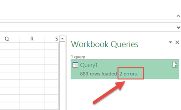
In the last post in this series, we worked with Date columns, namely our Birth Date column. After some transformation examples, we ended up preserving just the Year part of the that column and replacing our Birth Date column with a Birth Year column. Grand. However, when that query was saved, that were two rows that generated errors. Figure 1 shows this.

Figure 1
image

When there are errors resulting from a query, the number of errors will appear to the right of the Rows Loaded information in the Workbook Queries pane of the Power Query tab in Excel. The error information is not just informative. It also serves as a hyperlink to a special query filtered for just the error rows involved.

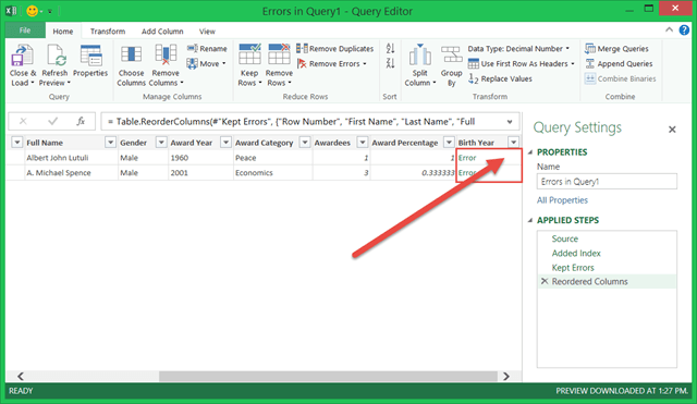
1. Click the “2 errors” hyperlink. This should launch a new query called Errors in Query1, as shown in Figure 2.

Figure 2
image

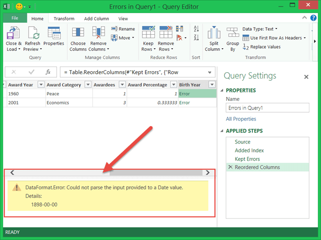
2. Click the white space to the right of the top “Error” value in the Birth Year column. This will reveal the error for that column on the row selected. The result should resemble what is shown in
Figure 3.

Figure 3
image

When you click on a row in a particular column, the contents of that cell appear in a new box at the bottom of the query window. If the selected cell is an Error cell, then the result is that the details of the error are revealed.

Note: You can also click on the Error value itself to get this information. However, that creates a new query step that filters for just that one row, making it difficult to look at more than one row quickly. So, I prefer to click next to the Error value instead as it makes it easier to go from one row to another.

In this case, the error is that Power Query could not isolate the Year value from “1891-00-00” as that value is not a valid date and therefore has no Year component.

3. Click the white space to the right of the Error value on the second row. That is shown in
Figure 4.

Figure 4

image

That looks familiar. Both of these records have the same problem. For the Nobel Laureate in question, the prize committee’s records included only the Year of birth, but not the exact date.

The good news is that, for our purposes, we only want the Year anyway. However, we will need to take some action in order for Power Query to capture the Birth Year values for these two Laureates.

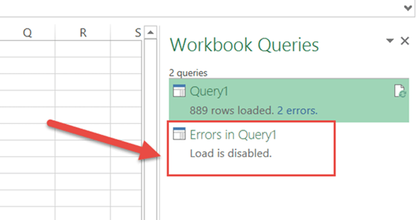
You will note that there are transformation options here in this Errors in Query1 query. If you make changes here to fix the errors and Close & Load this query, it will create a new query in your workbook that does not load anywhere but is accessible from other queries. The “Load is disabled” note will be explained in the next post on Loading Results. Figure 5 shows what it looks like after saving the Errors query.

NOTE: We will not be saving this Errors in Query1 query as part of this post. So, the next image is just for information and does not accompany specific actions you should take if you are following along.

Figure 5
image

This gives you the option of filtering the errors out of the Query1 query altogether (we will show that process later) and only dealing with them in the second, Errors in Query1 query. You could then append the cleaned up rows from the Errors in Query1 query to the Query1 query to bring them back into the dataset.

This ability is similar to the ability of SQL Server Integration Services to route Error rows along a different path so that the errors can be dealt with. While I have not done this much yet with Power Query, I very much appreciate having the option.

OK. Back to the example. Both of our errors have the issue that the proper Year value in their Birth Date is followed by “-00-00” which is certainly invalid for both the Month and the Day. The fact that their issues are identical is very convenient for us because it allows us to easily fix both errors with a single action.

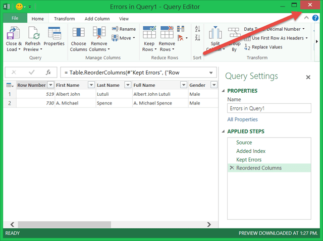
4. If you still have the Errors in Query1 query open, as shown in Figure 4, please click the X in the upper right of the query window, as shown in Figure 6, to close it.

Figure 6
image

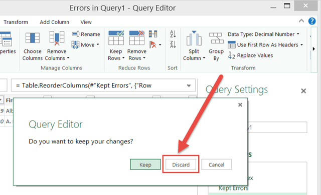
Power Query will know that the query has not been saved and will prompt you to do so, as shown in Figure 7.

Figure 7
image

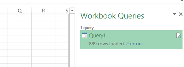
5. Since we do not want to keep a separate query for these errors, choose Discard, shown by the arrow in Figure 7. This will take us back to the Workbook Queries pane of the Power Query tab, as shown in Figure 8.

Figure 8
image

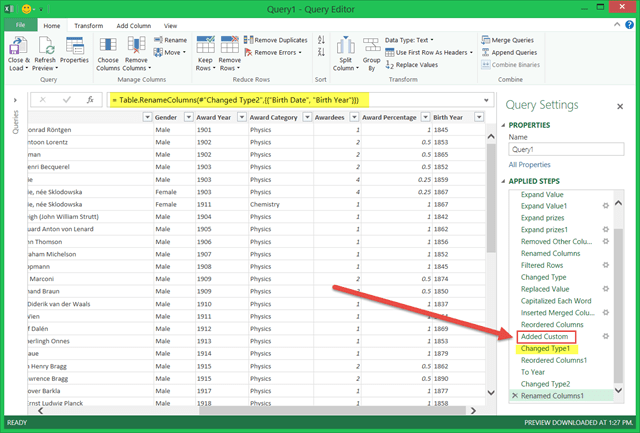
6. Double-click the Query1 query to open it. This will open the Query Editor, as shown in Figure 9.

Figure 9
image

The query will open to the final step, Renamed Columns1. However, at this step, the Birth Date column had already been converted to a Date. In order for Power Query to properly deal with our invalid dates, we must change the values for our two errors BEFORE the conversion to Date occurs. Since we changed Birth Date to a Date in the Changed Type1 step, shown highlighted in Yellow in Figure 9, we will have to insert a new step just before that, just AFTER the Added Custom step.

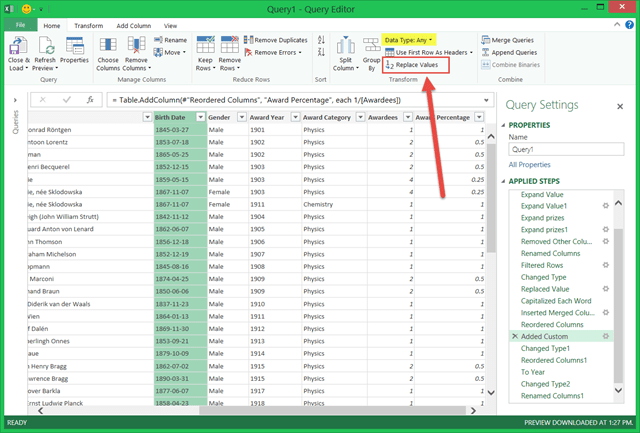
7. Click the Added Custom step in the APPLIED STEPS, shown by the arrow in Figure 9. This will change our Results Pane to the state of the query AFTER that step has been applied but BEFORE any subsequent step. This is shown in Figure 10.

Figure 10
image

Note that, as of this step, the Birth Date column is still of the Any data type. This is the perfect spot in the query for us to change some invalid date values to valid ones.

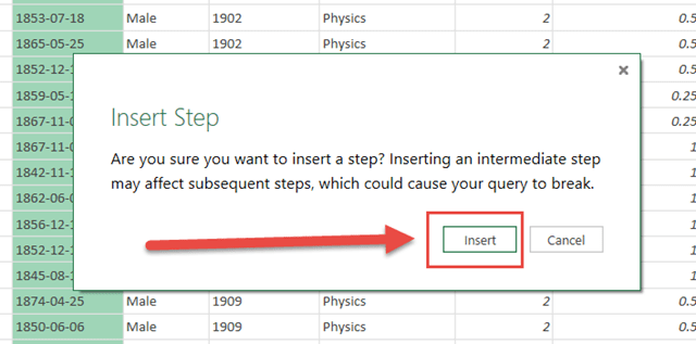
8. With the Birth Date column selected, click the Replace Values button, shown in Figure 10. This will reveal the warning shown in Figure 11. Note: There is a Replace Values button on the Transform tab as well. They work the same.

Figure 11
image

Since the steps in a query build upon each other, and have a specified order, adding new steps in the middle can cause issues. For example, if I add a new step here that removes columns, those columns will still be referenced in subsequent steps and those steps will become invalid and broken and unhappy. However, in our case, we are not making structural changes to our query, we are just replacing values in the data itself. So, we will be fine inserting our Replace Values step in the middle.

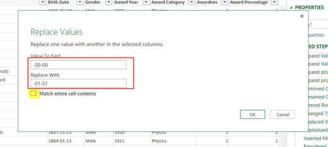
9. Click the Insert button shown by the arrow in Figure 11. This will activate the Replace Values dialog shown in Figure 12.

Figure 12
image

10. Enter “-00-00” in the Value to Find and “-01-01” in the Replace With boxes, respectively. Make sure the Match Entire Cell Contents box is NOT checked. The reason is that we only want to change the –00-00 parts of the values with –01-01. If we check that box, then Power Query will search for rows where the Birth Date columns contains the value –00-00. That would find zero results.

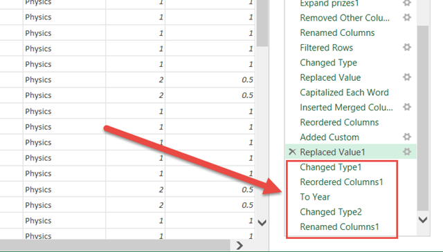
11. Click OK. The result should resemble Figure 13.

Figure 13
image

The benefit of taking this step will not be immediately apparent in the Results Pane. However, if you click through the steps following this new Replaced Value1 step, you should see that they all return data in the Results Pane. This means that there are no structural problems with any of those steps.

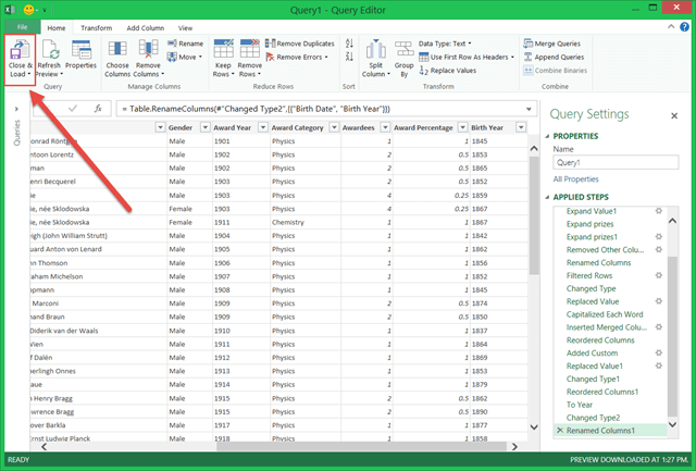
12. Click each step after Replaced Value1 in the APPLIED STEPS, shown by the arrows in Figure 13. The result of the final step, Renamed Columns1, is shown in Figure 14.

Figure 14
image

To make sure we have properly dealt with the two error rows, it is necessary for us to Close & Load the query.

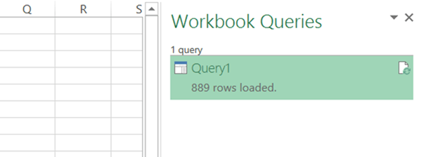
13. Click the Close & Load button shown by the arrow in Figure 14. This will execute query and return us to the Workbook Queries pane of the Power Query tab, as shown in Figure 15.

Figure 15
image

The absence of any mention of Errors shows that our fix worked.

Setting Up Errors

Sometimes, you will take steps that reveal errors right away in your dataset and you can actually see them in the Query Editor. This section will create some errors for us to use as examples.

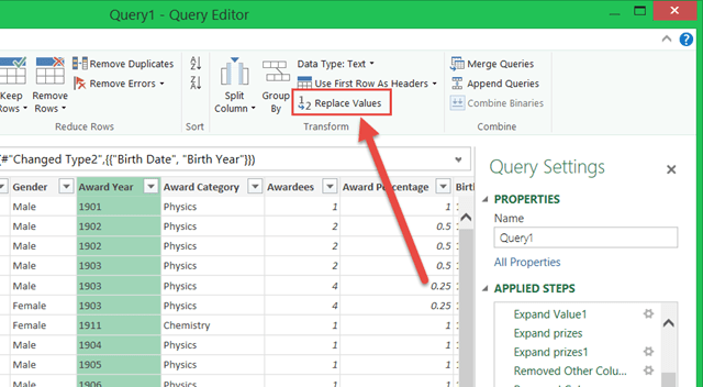
14. Double-click the Query1 query to open it in the Query Editor, as shown in Figure 16.

Figure 16
image

In this example, we will take specific steps cause some errors to show a few of the options available for dealing with rows that have errors in them. Our first step will be to modify some values in the Award Year column that will fail to convert to a whole number.

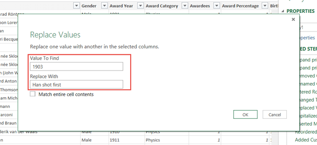
15. With the Award Year column selected, click the Replace Values button shown by the arrow in Figure 16. This will activate the Replace Values dialog we have seen before, as shown in Figure 17.

Figure 17
image

16. Type “1903” into the Value To Find box and a alpha text string of your choice in the Replace With box.

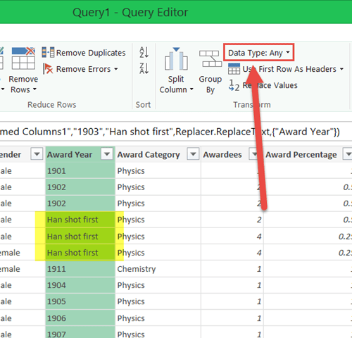
17. Click OK. The result should resemble Figure 18.

Figure 18
image

Note the text string we chose now appears in the Award Year column for the rows that contained 1903 as the Award Year. Also note that the Award Year column, which no longer contains values that are clearly one particular data type, has been converted to an Any data type by Power Query. This is something to keep an eye on. Even if you make specific data type assignments, subsequent actions could override that. You might be tempted to just avoid data type assignments until the last step of the query. However, you need to remember that some transformations are only available on columns of a specific data type. So, in reality, this is just something you need to watch out for. Double-checking at the very end to make sure columns have the types you want is not a bad idea.

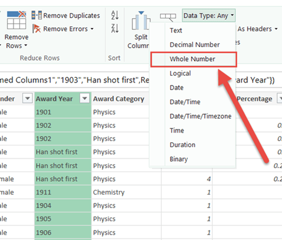
18. Click the Data Type button in the Transform section of the Home tab of the Ribbon, shown by the arrow in Figure 18. This will show the Data Type options in Figure 19.

Figure 19
image

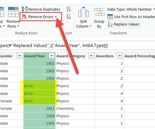
19. Choose Whole Number, as shown by the arrow in Figure 19. The results should resemble Figure 20.

Figure 20
image

Our text values failed to convert to a Whole Number and are therefore creating an Error state on those rows for the Award Year column.

When you have Errors in rows, you have a few options. These are found in two different places, which might seem counter-intuitive. However, since they behave quite differently, I can see what the decision was made.

Remove or Keep the Error Rows

You have the option of removing rows with an error state or even filtering your dataset to return only the error rows. Both of these options are found on the Home tab of the Ribbon in the Reduce Rows section.

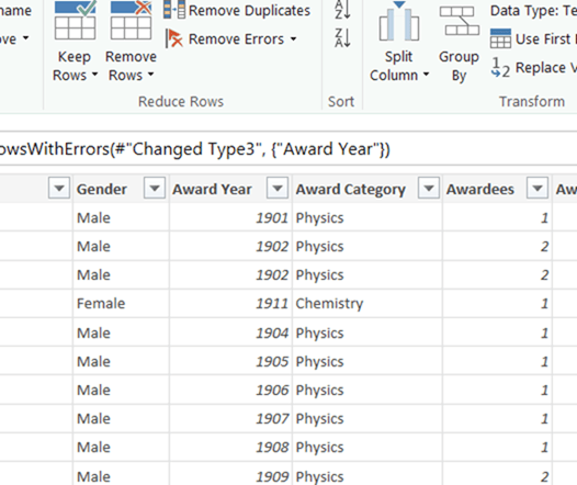
20. With the Award Year column selected, click the Remove Errors button, shown by the arrow in Figure 20. This will completely remove from the dataset any rows that have an Error in the Award Year column. The results should resemble Figure 21.

Figure 21
image

The error rows have been filtered out of the query and will no longer participate in any subsequent query steps or appear in the results that are loaded into Excel.

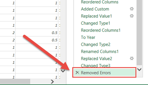
21. Click the X next to the shiny new Removed Errors query step, shown by the arrow in
Figure 22. This bring us back to the query we had in Figure 20, with the three error rows present.

Figure 22
image

Suppose we want to keep only the error rows and get rid of the rest of the rows.

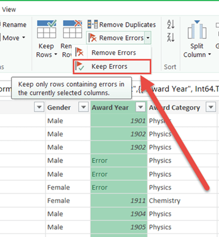
22. Click the tiny triangle on the right-hand side of the Remove Errors button, shown by the arrow in Figure 23.

Figure 23

image

Instead of just removing the error rows, which is the default operation performed when clicking the Remove Errors button, this will reveal the options shown in Figure 24.

Figure 24
image

You have the option of still just removing the errors. However, you also have the option to keep the error rows and dump the rest.

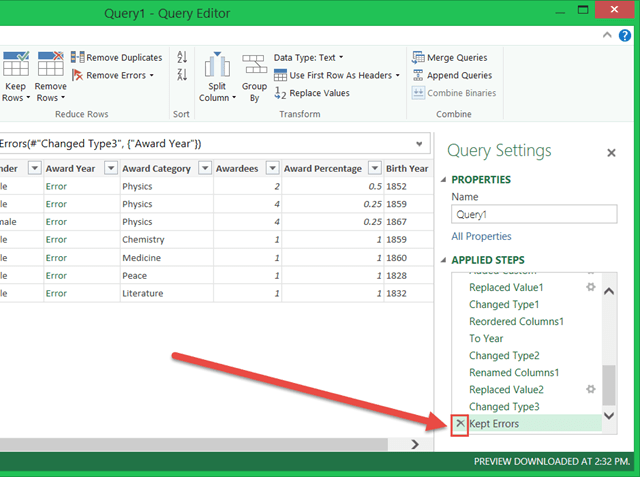
23. Choose Keep Errors, as shown by the arrow in Figure 24. This will produce the results shown in Figure 25.

Figure 25
image

The only rows left in our dataset are those that have an Error in the Award Year column. This shows that we had not sorted our dataset chronologically by Award Year since several 1903 rows were not visible before. We don’t want to keep this result, though.

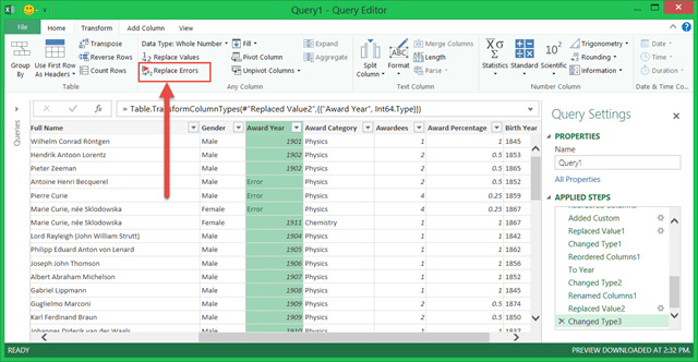
24. Click the X next to the Kept Errors step to delete it and return to the state shown in Figure 26.

Figure 26
image

Replace Errors

You also have the option to replace the Error state with a specific value that you specify. This is similar to the Replace Value option, but instead of specifying a Value to Find, Power Query just looks for the Error state. This option is on the Transform tab.

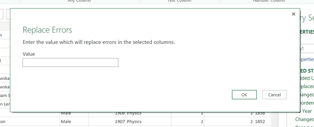
25. With the Award Year column selected, click the Replace Errors button in the Any Column section of the Transform tab. This will activate the Replace Errors dialog as shown in Figure 27.

Figure 27
image

From here, you can decide what single value to use in place of your errors. The value you choose will replace every instance of the Error on the selected column(s) and must match the data type of the column(s). For example, a blank (no value), is considered to be of the Text data type by Power Query. Since the Award Year column in this example has been converted to a Whole Number, a blank will not be accepted here.

26. Leave the Value textbox empty and click OK. The result is shown in Figure 28.

Figure 28
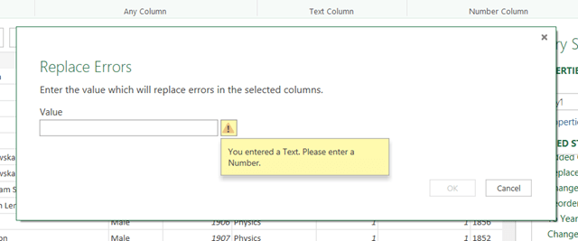
image

Today, the role of HAL 9000 will be played by Power Query: “I’m sorry, Dave. I’m afraid I can’t do that.”

This means that you will sometimes have to give some thought when deciding when and how to deal with errors.

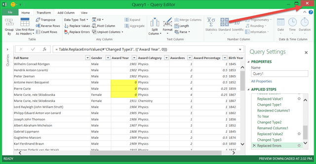
27. Enter 0 for the Value instead of leaving it blank.

28. Click OK. The result should resemble Figure 29.

Figure 29
image

The errors rows remain, but their values have been changed to a value that does not produce and Error state. Grand.

Back in Step 13, we saved the Query1 after fixing those two error rows in Birth Year. Everything we have done since then was just to show how to deal with errors we specifically created. At this point, we can just close the query and discard changes and we will be ready for the next post in the series.

29. Click the X in the upper right corner of the Query Editor to close it.

30. Choose Discard from the screen that follows.

That takes care of dealing with Errors. In the next post, we will talking about Loading results to Excel.

Power Query Decathlon – Beginner 07: Date Columns

NOTE: This post was created using the November 2014 version of Power Query. In later versions, some of the screens or functionality could be different.

You can download the Excel 2013 file necessary to perform the steps in this post here. To get to the existing query, click the Workbook Queries button on the Power Query ribbon.

In this post, we will play with transformation options available for Date typed columns. Our starting point is shown in Figure 1.

NOTE: Because my regional settings for Windows are set to English – United States, my default format for dates is mm/dd/yyyy. So, in this post, my dates will follow that format. The functions in Power Query will work appropriately for your region.

Figure 1

image

The Birth Date column still has the Any data type. Our first course of action will be to change its type to Date.

1. With the Birth Date column highlighted, click the Data Type option on the ribbon (on either the Home or Transform tabs). This will reveal the options shown in Figure 2.

Figure 2

image

2. Choose Date. The result will resemble Figure 3.

Figure 3

image

Note that the values in the column have become right-justified, are now italic, and the hyphens between the date parts have changed to slashes. Also, you will notice that the final query step in the APPLIED STEPS section is still Changed Type1. Since the last step performed in the last post was to change the data type of the Award Percentage column to a decimal number, and the first of this one is to change the type of the Birth Date column to a Date, Power Query merged both of those changes into a single step.

Since we will want to keep the Birth Date column while we play with the various options, we will be adding new columns. New columns are added to the far right of the query. So, our next course of action will be to move the Birth Date column to the end to make it easier to view it alongside the new columns.

3. Right-click the Birth Date column to expose the menu shown in Figure 4. Note, if you are using a device with no Right-click option, you can also use the Move button on the Home tab of the ribbon.

Figure 4

image

4. Choose “To End” as shown in Figure 4. The result will resemble Figure 5.

Figure 5

image

The Birth Date column is now at the far right of the query, after Award Percentage.

5. With the Birth Date column selected, click the Date button in the From Date & Time section of the Add Column tab of the ribbon, as shown in Figure 5. This will reveal the options shown in Figure 6.

Note: It is important to use the Add Column tab here so that our transformation will create a new column instead of replacing the existing one.

Figure 6

image

As dates have multiple parts, there are separate functions you can use for dealing with each part.

Let’s create a new column that returns the Month part of the date.

6. From the Month menu shown in Figure 6, choose Month, shown by the arrow in Figure 7.

Figure 7

image

The result will be a new column, called Month by default, to the right of the Birth Date column, as shown in Figure 8.

Figure 8

image

Note that this returns the ordinal number for the month, not a name. In Figure 8, I am showing the Home tab in order to highlight the fact that the Month transformation also performed the added work of converting the resulting column to the Decimal Number data type.

7. Since we will not be keeping this column, click the X next to the Inserted Month query step, as shown in Figure 9.

Figure 9

image

This will take our query back to the way it was in Figure 6, shown again below as Figure 10.

Figure 10

image

In addition to finding the parts of a date, you can also find other values based on that date. For example, you can use a date value to find the last day of that month. This could be useful in situations where the number of days in a month will matter. This functionality is easier than building logic to determine which years were leap years (ah, February) and then building the End Date column from there.

8. From the Date menu on the Add Column tab, choose Month –> End of Month, as shown in Figure 11.

Figure 11

image

The result is shown in Figure 12.

Figure 12

image

Note that the transformation also correctly typed the resulting column as a Date.

We do not want to keep this column, so we will delete this step.

9. Click the X next to the Inserted End of Month step in the APPLIED STEPS, as shown by the arrow in Figure 13, to delete it.

Figure 13

image

This will, once again, take us back to the state of the query in Figure 6, as shown in Figure 14.

Figure 14

image

I used this dataset for a demo in which I wrote the result to the Excel Data Model (we will cover that in a future post). One thing I had not though about was that the earliest value supported for a Date column in Power Pivot is January 1, 1900. You can see from the data that there are many Nobel Laureates who made the the inconvenient decision to be born prior to 1900. The nerve of some people… 🙂 For that reason, I determined it was best to just use the Birth Year of each Laureate instead of the full date. To clarify, we want to replace the Birth Date column with a Birth Year column.

10. With the Birth Date column selected, click the Date button in the Date & Time Column section of the Transform tab of the Ribbon, as shown in Figure 14. This will reveal the familiar Date options shown in Figure 15.

Figure 15

image

11. Choose Year from the Year option. This will produce the result shown in Figure 16.

Figure 16

image

Figure 16 shows the Home tab in order to highlight the Data Type.

Since we used the Transform tab instead of the Add Column tab, the existing Birth Date column containing the full date was replaced with a Birth Date column containing just the Year part of the Birth Data. Note that the data type was changed to a Decimal Number. We have a few issues with this result. First, the name of the column no longer makes sense for the content it holds. And second, we will never ever want to perform math on these values, so a text data type would be more appropriate in order to prevent mathematical operations that have no hope of being valid.

12. On the Home or Transform tabs, change the data type of the Birth Date column to Text, as shown in Figure 17.

Figure 17

image

Notice that the values in the column are now left-justified.

13. Right-click the Birth Date column header, and choose Rename, as shown in Figure 18.

Figure 18

image

Note that you can also double-click the column heading or use the Rename button in the Manage Columns section of the Home tab to rename this column.

14. Name the column Birth Year. The result should resemble Figure 19.

Figure 19

image

If you want to save this query and file for use in the next post, go for it. If you do, you should notice that there are two errors found, as shown in Figure 20.

Figure 20

image


Those will be dealt with in the next post, which covers handling errors.

Power Query Decathlon – Beginner 06: Number Columns

NOTE: This post was created using the November 2014 version of Power Query. In later versions, some of the screens or functionality could be different.

An apology: I want start this post by apologizing for making it harder to follow this series than I should have. Rather than put the onus on you, dear reader, to maintain the working file for each post, I should have just supplied the necessary source file at the beginning of each post. I have hereby rectified that on all previous posts in this series and will provide the work file for each post from here on.

You can download the Excel 2013 file necessary to perform the steps in this post here. To get to the existing query, click the Workbook Queries button on the Power Query ribbon.

While I tend not to do much with number columns in Power Query other than formatting, I wanted to make sure to provide an example to show that you certainly CAN work with them. There are certainly occasions where doing math in Power Query makes sense. I have just not encountered many yet.

We start the the query shown in Figure 1.

Figure 1

image

Our sole number column in this query is the Awardees column, shown highlighted in Figure 1. This fields contains the number of people that shared each portion of a particular Nobel Prize. We will start out with something basic.

Information

The Information button, in the Number Column section of the Transform tab and the From Number section of the Add Column tab, has three options. The options are shown in Figure 2.

Figure 2

image

The Is Even option returns the value TRUE if the number is an even number and FALSE if the number is odd. The Is Odd option does the opposite, returning TRUE for odd numbers and FALSE for even ones. Contrary to what you might think, the Sign option is not related to Tesla OR the “Wormsign” cry from Dune. It actually returns a –1 for negative numbers and a 1 for positive numbers.

Our first example will be to use the Sign option. In order to make it worthwhile, we will first use the Replace Values transformation to make some of our values negative.

1. With the Awardees column highlighted, click the Replace Button on the Home tab of the ribbon, shown in Figure 3. Note: The Replace Values button on the Transform tab will work just fine as well.

Figure 3

image

This will activate the Replace Values dialog, as shown in Figure 4.

Figure 4

image

2. Enter 1 in the Value To Find and –8675309 in the Replace With boxes, respectively, as shown in
Figure 4. Thanks to Jenny for the number.

3. Click OK. The result will resemble Figure 5.

Figure 5

image

Notice the presence of –8675309 values where the 1 values used to be. Note also that doing this causes the Awardees column to change to the Any data type. Interesting. Even though the new value is still a whole number, the use of an Any Column transformation will convert that column to the Any data type. You can see this in Figure 6.

Figure 6

image

4. Making sure the Awardees column is selected, click the Data Type option and change it to Whole Number.

5. Click to select the Awardees column again.

6. Click the Sign option of the Information button on the Add Column tab of the ribbon, as shown in Figure 7.

Figure 7

image

Since we chose the Add Column tab from which to perform this action, the result will be a new column containing the results of the Sign transformation, as shown in Figure 8.

Figure 8

image

Notice that all of the rows with a negative value for Awardees have a –1 value for the Sign column.

Since we don’t want to keep the work from this example, we will delete these steps to return to our starting point.

7. Delete the last three steps in the APPLIED STEPS, as shown in Figure 9.

Figure 9

image

Like Math and Stuff

For this example, we will use the values in the Awardees column to calculate the percentage of the Nobel Prize won by each Laureate. Take a close look at Figure 10.

Figure 10

image

For the 1903 Nobel Prize for Physics, we see there are three Laureates. However, at first glance, the values seem a bit confusing. A little research cleared that up, though. Antoine Henri Becquerel won 1/2 of that prize while Pierre Curie and Marie Curie split the other half, getting 1/4 each. Interesting, eh? The More You Know.

This means we can use the value in the Awardees field to calculate what percentage of each Nobel Prize was awarded to each Laureate.

8. Click the Add Custom Column button on the Add Column tab of the ribbon, as shown in
Figure 11.

Figure 11

image

This will launch the dialog shown in Figure 12.

Figure 12

image

9. Name the new column something sensible, like Award Percentage.

10. Type “1/” in the Custom Column Formula box.

11. Scroll down in the Available Columns box until Awardees becomes visible.

12. Click on Awardees to select it.

13. Click the Insert button, shown by the arrow in Figure 13.

Figure 13

image

Once you have completed these steps, the Add Custom Column dialog should resemble Figure 14.

Figure 14

image

The formula is 1/[Awardees]. This means that, for each row, this new column will be equal to the result of dividing the value 1 by the value in the Awardees column in that row.

14. Click OK. The result is shown in Figure 15.

Figure 15

image

As we would expect, the values make sense as Mr. Becquerel has 50% and the Curies each have 25%. Grand.

The Award Percentage column defaults to the Any data type. Let’s make it something more appropriate.

15. Click the Award Percentage column to select it.

16. Click the Data Type option on either the Home or Transform tabs. The Transform tab option is shown in Figure 16.

Figure 16

image

17. Select Decimal Number as the data type.

The final query for this example will resemble Figure 17.

Figure 17

image

If you are following along with your own file, you can click Close & Load to save this query and then save the file for next time. Otherwise, you can just use the source file I will provide at the beginning of that next post, in which we will play with Date Column options.

Power Query Decathlon – Beginner 05: Text Columns

NOTE: This post was created using the November 2014 version of Power Query. In later versions, some of the screens or functionality could be different.

You can download the Excel 2013 file necessary to perform the steps in this post here. To get to the existing query, click the Workbook Queries button on the Power Query ribbon.

As discussed in the last post in this series, Power Query Decathlon – Beginner 04: General Transformations, the transformations on the Transform tab in Power Query are arranged in meaningful groups, largely driven by the data type of the column in question. If you have not done so, follow the steps in that post in order to be ready to follow along.

In this post, we will focus on the transformations available for Text columns, shown by the arrow in Figure 1.

Figure 1

image

Format

The Format transformations deal with capitalization, spaces, and non-printing characters. The options and their descriptions are as follows:

“lowercase”: makes all of the letters in the selected text column(s) lowercase

“UPPERCASE”: makes all of the letters in the selected text column(s) UPPERCASE

“Capitalize Each Word”: makes the first letter in each word of the selected text column(s) UPPERCASE and all other letters lowercase

“Trim”: removes any leading and trailing spaces from the values in the selected text column(s)

“Clean”: removes any non-printable characters from the values in the select text column(s)

The one we will demonstrate in this post is the Capitalize Each Word transformation. Figure 2 shows that the values in the Gender and Award Category columns are lowercase. While this is not an issue with understanding, it may be more appealing for users if the values were capitalized instead.

Figure 2

image

1. Select both the Gender and Award Category columns.

2. Click the Format button on the Ribbon.

3. Choose the “Capitalize Each Word” option, as shown in Figure 3.

Figure 3

image

The results of this transformation are shown in Figure 4.

Figure 4

image

Hazzah!

Merge Columns

Merging columns involves combining the values from more than one column into a single column. There are actually two different results you can achieve when merging columns. The first is to replace all of the merged columns with the new column. With this option, the original columns go away. The second is a create a brand new column with the merged values while leaving the original source columns intact. We will start with option 1.

4. Select both the First Name and Last Name columns.

5. Click the Merge Columns button on the Transform tab of the Ribbon, as shown in Figure 5. NOTE: The Merge Columns button is grayed out by default. It is only activated when more than one column is selected.

Figure 5

image

After clicking the Merge Columns button, the dialog shown in Figure 6 will appear.

Figure 6

image

In this dialog, you have the option to choose a separator for the values in the resulting column. You also have the ability to choose the name of that column.

6. Name the column something appropriate, like Full Name.

7. Click the Separator drop down. This will display the options shown in Figure 7.

Figure 7

image

8. Choose Space. This will, as you might expect, separator the values from each column with a space. The dialog should now look like Figure 8.

Figure 8

image

9 Click OK. This will result in what appears in Figure 9.

Figure 9

image

Note that the First Name and Last Name columns have been replaced by the new Full Name column. In this example, we will assume that is NOT what we want.

10. Delete the Merged Columns step, shown by the arrow in Figure 9.

This time, we will create the Full Name column while preserving the First Name and Last Name columns.

11. Select both the First Name and Last Name columns, just as we did before.

12. Click the Add Column tab of the Ribbon, shown by the arrow in Figure 10.

Figure 10

image

The Add Column tab has some options that are available on other tabs, and a few that are only available here. Figure 11 shows the Add Column tab.

Figure 11

image

While we will not go into them in this series, I will take a quick moment to discuss one of the options here. The Add Custom Column button allows you to create a new column manually with M code. As of the November 2014 release of Power Query, the dialog for the Add Custom Column is not very robust. But let’s give the team some time. They are doing great work.

13. Click the Merge Columns button on the Add Column tab, shown by the arrow in Figure 11.

14. The steps for creating the new column on the Add Column tab are identical to the steps on the Transform tab, other than the tab on which you click the button. Follow the same steps as before, specifying the Space for the separator and a meaningful name like Full Name, as shown in Figure 12.

Figure 12

image

15. Click OK. The result should resemble Figure 13.

Figure 13

image

Note that the new column is added to the end, the far right, of the query. I did scroll to the right before capturing Figure 13 in order to see the new column. We have ability to move it elsewhere, though.

16. Right-click on the Full Name column to reveal the context menu shown in Figure 14.

Figure 14

image

17. Click Move.

18. Click To Beginning, as shown in Figure 14. NOTE: If you are using a device without the option for right-clicking, you can also just select the column and use Move button in the Manage Columns section of the Home tab. However you accomplished the move, the result will appear in Figure 15.

Figure 15

image

I did scroll to the left before capturing Figure 15 to see the Full Name column in its new position. The Move options are great when you want to move something a long way, like when you have a lot of columns. When you want to move columns within your field of view, you can just click and drag them.

19. Click and drag the Full Name column until the indicator shows it can be dropped to the right of the Last Name column, as shown in Figure 16, and release it.

Figure 16

image

The result will be that the Full Name column is now positioned between the Last Name and Birth Date columns, as shown in Figure 17.

Figure 17

image

Note that Power Query still put both of the column moves into a single step, even though we used two different methods to accomplish them. Cool.

Split Column

The last transformation we will cover in this post is the Split Column. This allows you to divide a single column into two or more columns based on a delimiter you specify or a number of characters. In this example, we will split the Birth Date column into 3 columns, with the splits occurring on the “-“ between the components of the date value.

20. Select the Birth Date column. NOTE: Our Birth Date column is still of the Any data type at this point. However, the Split Column transformation will still work just fine.

21. Click the Split Column button on the Transform ribbon, shown by the arrow in Figure 18.

Figure 18

image

This will reveal the two options shown in Figure 19.

Figure 19

image

22. Click the By Delimiter option shown by the arrow in Figure 19. This will open the Spit Column dialog shown in Figure 20.

Figure 20

image

These are the default options. These options will look for commas and, due to the active option under Split, create a new column after each comma. In our case, the comma delimiter will not help.

23. Click the delimiter drop down, shown by the arrow in Figure 20. This will reveal the pre-populated options shown in Figure 21.

Figure 21

image

The hyphen, the separator between the parts of the value in our Birth Date column is not available in this list. No worries.

24. Click the “Custom” option, shown by the arrow in Figure 21. This will activate a textbox allowing you to enter the delimiter character(s) you need.

25. Enter in a hyphen, as shown in Figure 22.

Figure 22

image

The next choice we have to make is in the Split section. The options are pretty self-explanatory. For our example here, the default option, “At each occurrence of the delimiter,” is the one we want.

26. Click OK. This will produce the result shown in Figure 23.

Figure 23

image

There are a few things to note here. First, because we chose the Split Column button on the Transform ribbon, the original Birth Date column is gone. Second, the delimiter itself, the hyphen in our example, is not persevered. Third, for better or worse, Power Query has chosen not only to split the column, but also to change the data type of the resulting columns to Whole Number since they seem to match that pattern. So, this is a case where a single action generated TWO query steps. If the data type change is not appropriate, you can delete that step and still keep the split columns.

Note: The reason that final step is called “Changed Type 1” is that we already had a step called “Changed Type.” When there must be more than one instance of the same transformation, Power Query will merely add an increment number to the name since the names of steps MUST be unique within a query. The reason for this is that the steps behind the scenes in the M code reference previous steps by name. If there is more than one step with the same name, the M code will freak out as it could not know which one is correct.

The last thing we need to do in this post is to undo the split column, since we don’t need that going forward.

27. Delete both the Changed Type 1 and Split Column steps shown by the arrow in Figure 23. The result will be just like Figure 17 above, with the Full Name column having been created and moved into position just to the right of the Last Name column. This is shown in Figure 24.

Figure 24

image

That wraps up our work with Text Columns. In the next post in the series, we will start working with Number Columns. If you want to follow along, please use the Close & Load button to save this query and then save the Excel file. We will continue to use it in upcoming posts.

Power Query Decathlon – Beginner 04: General Transformations

NOTE: This post was created using the November 2014 version of Power Query. In later versions, some of the screens or functionality could be different.

You can download the Excel 2013 file necessary to perform the steps in this post here. To get to the existing query, click the Workbook Queries button on the Power Query ribbon.

It is time to start covering Transformations. These are what really help set Power Query apart from the capabilities offered by Power Pivot. Power Pivot has long had a respectable list of sources you could use. However, it has never provided the ability to transform/shape/modify data before pulling it into the data model. Sure, you could do that sort of thing in source queries, but that only helps when pulling data from a source that directly supports queries, like a database. With Power Query, once you have pulled data from a source, you have a lot more work you can do before sending it to its final destination (reference to terrible movie franchise not intended).

While there are Transformations available to you from the Home tab of the Query Editor, the full list of available options is available on the Transform tab. For this post, we will focus on the Transformation tab.

1. Click the Transform tab heading as shown in Figure 1.

Figure 1

image

This will expose the Transform tab of the Ribbon, as shown in Figure 2.

Figure 2

image

As you can see in Figure 2, the available Transformations are organized into the following groups:

  • Table
  • Any Column
  • Text Column
  • Number Column
  • Date & Time Column

For this post, we will show examples from the first two options, Table and Any Column.

Table Transformations

Table Transformation, as their name suggests, operate on the table as a whole. Figure 3 shows a closer look at those options.

Figure 3

image

The Use First Row as Headers option is pretty straightforward and we have already seen that in the post on importing data. We will not cover it again here.

For now, we will start with the Group By transformation. This is useful when you have a table of detail data that you want to summarize in some way. For this example, we will use the Group By transformation to return a list of the Nobel Laureates that have one more than one Nobel Prize.

We will start with the query we saved from last time, as shown in Figure 4. If you have not done so, you will need to follow the steps in the previous post, Power Query Decathlon – Beginner 03: Managing Columns and Rows, to create the query show in Figure 4.

Figure 4

image

2. Using whatever method you like, select both the First Name and Last Name columns. The main option in Windows is to hold down the Ctrl key while clicking each column in succession.

3. Once they are selected, click the Group By button on the Ribbon, as shown in Figure 5.

Figure 5

image

Doing this will activate the Group By dialog shown in Figure 6.

Figure 6

image

The Group By section shows the columns we will be grouping by, First Name and Last Name. Notice there is a + to the right of Group By. This is so that we can add additional columns do group by. Since we selected the two columns manually, they both added themselves for us.

The New Column Name toward the bottom shows the new aggregation that will be performed as part of this Group By. The default is to perform just a count of rows according to the Group By columns. In our case, each row represents and awarding of the Nobel Prize, so this default is just fine. Note that you can also choose NOT to add any new columns, and merely produce a distinct list. If you want to do that, you can click the – to the right of the Count column. This will remove that entirely. For now, we will just specify a different name for our new column.

4. Change the New Column Name value, shown by the arrow in Figure 6, to read Award Count.

5. Click OK. This will perform the transformation and produce a result like the one shown in    Figure 7.

Figure 7

image

6. Click the filter button for the Award Count column, shown by the arrow in Figure 7. This will produce the filter dialog for that column, as in Figure 8.

Figure 8

image

The filter dialog shows that no Laureate (person or organization) has ever won more than 3 Nobel Prizes (at the time of this writing, anyway). Interesting.

7. Click the checkbox next to 1, shown by the arrow in Figure 8, to deselect it. At this point, 2 and 3 should stay selected.

8. Click OK. This should produce a result similar to Figure 9.

Figure 9

image

Cool. The International Committee of the Red Cross has won 3 Nobel Prizes. Good on ya. Marie Curie is listed as well. She was actually the first person to win two. That rules.

That is the Group By transformation in a nutshell. Before we continue, we will want to go back to what we had in Figure 4.

9. Click the X next to both the Filtered Rows 1 and Grouped Rows steps, as shown by the arrow in Figure 9. Note: The X will appear for the Grouped Rows step once it has focus. This will bring us back to the beginning, as shown in Figure 10.

Figure 10

image

The Transpose transformation will basically pivot all rows into columns. There are enough rows currently in this dataset that we end up losing data while doing this. So, we will not be showing an example of it. But feel free to play around with Transpose on a smaller set of data.

Any Column Transformations

When data first comes into Power Query from a source that is not strongly typed, like a text file or the API that is the source for this query, columns will have the Any data type. This is not a type that you can assign. Rather, it is the one Power Query uses when it cannot be sure of the data type for a column. To see the data type for a column, highlight the column and look at the top of the Any Column transformation box, shown in Figure 11.

Figure 11

image

In fact, if you examine the data type for each column in the query, they are all Any at this point. One of the things that is often done during the transformation of data is to change the data type of columns. Perhaps you have dates stored as numbers in your source and need them to actually be Dates to enable calendar-based calculations. Or perhaps you have a numerical value stored as text in a file and you need to convert it to an actual number in order to perform mathematical calculations.

10. Select the First Name, Last Name, Gender, Award Year, and Award Category columns.

11. Click the Data Type drop-down and select Text, as shown in Figure 12.

Figure 12

image

In case you are wondering, Yes, I am making the Award Year a text column. Why? Well, when will it EVER make sense to do math with this column? Will I SUM it? Average it? Heck no. So, since it will never make sense as a participant in a mathematical calculation, I will prevent my end users of the resulting data model from attempting it by making it a Text column. Decisions like this are a good example of helping to save end users from themselves.

12. Click the Awardees column to select it.

13. Click the Data Type option and set it to Whole Number, like in Figure 14. This field contains the number of awardees that shared any particular awarding of a Nobel Prize. Since this is a Count, it will make sense to perform mathematical operations with it. Thus, we make it a Whole Number.

Figure 13

image

Since we have made these data type changes in succession, I want to call your attention to the fact that Power Query was smart enough to put them into a single step rather than one for each change. The APPLIED STEPS shown in Figure 15 show that effectively.

Figure 15

image

The last transformation we will cover in this post is the mighty Replace Values transformation. This allows you to search the values in a column and replace one particular value with a different value you specify. The new value must be of the same data type as the replaced value and will replace every instance of the search value with the new value specified. Since it works on every data type (as far as I have determined, anyway), it makes sense that Microsoft chose to place this in the Any Column transformations section of the Ribbon.

14. Click the filter button for the Birth Date column, shown in Figure 16.

Figure 16

image

This will activate the Filter dialog for that column, shown in Figure 17.

Figure 17

image

Note the value by the arrow. This value is not a valid date. So, when we try to convert this column to a date, we will get errors on any row with this value.

15. Click the Cancel button to close the filter dialog.

16. Make sure the Birth Date column is selected.

17. Click the Replace Values button on the Ribbon, shown by the arrow in Figure 18.

Figure 18

image

This will open the Replace Values dialog shown in Figure 19.

Figure 19

image

Enter “0000-00-00” into the Value To Find box and leave the Replace With box empty. The dialog should look like Figure 20.

Figure 20

image

18. Click OK.

19. Click the Filter button on the Birth Date column again. It should resemble Figure 21.

Figure 21

image

In place of the (0000-00-00) value, we have a blank. This will play much better when we convert this to a Date column later. NOTE: There is a good reason we are not converting the Birth Date column to be a Date type in this post. So, if you want to continue to follow along, please leave the Birth Date column as the Any data type for now.

20. Click the Home tab heading to return to that tab.

21. Click the Close & Load button, shown in Figure 22, to save this progress.

Figure 22

image

In the next post, we will show examples of what you can do with Text columns.

Power Query Decathlon – Beginner 03: Managing Columns and Rows

NOTE: This post was created using the November 2014 version of Power Query. In later versions, some of the screens or functionality could be different.

You can download the Excel 2013 file necessary to perform the steps in this post here. To get to the existing query, click the Workbook Queries button on the Power Query ribbon.

Once you have a query pointed at a source in Power Query, it is a good time to select just the columns and rows you actually want to work with. I would strongly advise against the “just pull everything” philosophy. Any processing you do on data you are just going to get rid of later is wasted processing and wasted time.

Managing Columns

If you have not done so, and wish to perform the steps in this post, please follow the steps in the From Web section of the previous post, Power Query Decathlon – Beginner 02: Importing Data. This example will start there as a foundation. Figure 1 shows our starting point.

Figure 1

image

There are a few different methods for selecting columns. The first we will show is the Choose Columns option.

1. Click the Choose Columns button on the Query Editor Ribbon, shown by the arrow in Figure 1. This will activate the column chooser, as shown in Figure 2.

Figure 2

image

Even in this one screen, there are a few options. If you only want a small subset of the columns available, you can click the checkbox next to (Select All Columns) to deselect all columns and then click the checkbox for the columns you want. Or you can click the checkbox to deselect the columns you don’t want.

2. With the method of your choice, ensure that only the columns shown in Figure 3 are selected and click OK. We will not be using the others.

Figure 3

image

Once you have clicked OK, your Results pane should resemble Figure 4.

Figure 4

image

Note that the columns that were NOT checked have been removed. We also have a new step listed in the APPLIED STEPS.

In the previous post in the series, I recommended that you rename objects as soon as you can. Now the we have removed the columns we don’t want, this is a good time to make sure all the remaining columns have the name we want them to have.

3. Right-click on the “firstname” column to reveal the menu shown in Figure 5.

Figure 5

image

4. Choose Rename. This will put the column name in edit mode, as shown in Figure 6.

Figure 6

image

5. Change the name to First Name and hit the <Enter> key. The result will resemble Figure 7.

Figure 7

image

6. Rename the other columns until the have the names you want. The names I chose are shown in Figure 8.

Figure 8

image

As long as you take no other actions in between the renaming of the columns, Power Query will combine all of the renaming actions into a single query step. Schweet.

You can also rename columns by highlighting the column and clicking the Rename button on the Query Editor ribbon, as shown in Figure 9.

Figure 9

image

This is a good option when you are using a device where right-clicking is challenging or impossible. I pretty much always have the option to right-click so I just use that.

We can also change our column selection by using the Remove Columns button. That button and its underlying options are shown highlighted in Figure 10.

Figure 10

image

The first option, Remove Columns, will remove all currently select columns. This is also the default behavior of the Remove Columns button itself.

7. Use Ctrl-Click to select the First Name and Last Name columns, as shown in Figure 11.

Figure 11

image

8. Click the upper half of the Remove Columns button. The result will be that the First Name and Last Name columns will be removed from the query, as in Figure 12.

Figure 12

image

Great. Those columns are gone. However, we will actually want them. So, we will need to undo that action. Notice the Remove Columns step that is shown by the arrow in Figure 12. This is the step that removed those columns.

9. Click the X-shaped thingy-bobber for Removed Columns to delete that step. The result should resemble Figure 13.

Figure 13

image

You also have the option to remove all columns EXCEPT the ones you have selected. This is a great option when your source has a lot of columns and you only want a few of them.

10. Ctrl-click the First Name and Last Name columns to select them both, as shown in Figure 14.

Figure 14

image

11. Click the bottom half of the Remove Columns button, as shown in Figure 14. This will expose the Remove Other Columns option shown in Figure 15.

Figure 15

image

12. Click the Remove Other Columns option. This will remove all columns EXCEPT the First Name and Last Name, as shown in Figure 16.

Figure 16

image

Since we actually DO want those removed columns, we can undo this action by clicking the X next to Removed Other Columns shown by the arrow in Figure 16. This will return us to situation shown in Figure 17.

Figure 17

image

That is all we will cover for Managing Columns. We will cover moving columns around in a future post. Let’s move on to Rows.

Managing Rows

In Power Query, you have the ability to to filter rows based on the values that live in columns. For example, in the dataset we are using for the example, There are some rows that don’t have a value at all in the First Name column. That absence of a value appears in the dataset as (null). In that case, we want to remove the row entirely.

13. Click the triangle to the right-hand side of the column header for First Name, as shown by the arrow in Figure 18.

Figure 18

image

This will expose the Filter dialog for that column, shown in Figure 19.

Figure 19

image

To verify that the rows with the (null) in the First Name are actually rows we want to exclude, we can temporarily filter for just those rows.

14. Click the (Select All) to deselect all of the values.

15. Click the checkbox next to (null) so that ONLY that value is selected. Your filter dialog should resemble Figure 20.

Figure 20

image

16. Clock OK to apply that filter to the dataset. This will only keep rows that have a (null) for the First Name field. All other rows will be removed. This should resemble Figure 21.

Figure 21

image

It is pretty obvious that these rows provide no value to us. Therefore, we can conclude that filtering them from the dataset is probably a good idea.

We have a few options for doing this. We can delete the Filter Rows step like we have deleted steps before. However, we could also merely reconfigure the filter on that step.

Note: Query Steps build on each other. Renaming a step in the middle is likely to result in subsequent steps breaking as they would reference the original name of the step and not the new name. In this example, we have no subsequent steps, however, I feel it is important to show you how to change an existing step so you know you have that option when you need it.

17. Click the gear icon to the right-hand side of the Filtered Rows step, shown by the arrow in Figure 21. This will launch a different filter dialog than we have seen before. That new dialog is shown in Figure 22.

Figure 22

image

Right now, our query is filtered to only return rows where the First Name column EQUALS null. We want to make the exact opposite choice, ie we only want to keep rows where the First Name column  DOES NOT EQUAL null.

18. Click the triangle to the right-hand side of the equals operator, shown by the arrow in Figure 22. This will expand to show all of the operators we have available to us, as in Figure 23.

Figure 23

image

23. Click the “does not equal” value from the list so that the dialog now looks like Figure 24.

Figure 24

image

24. Click OK to commit the change to the Filtered Rows step. Your query should not resemble Figure 25.

Figure 25

image

If you like, you can click the arrow icon (now shown with a filter icon as well) in the First Name column header to see that all values EXCEPT (null) are selected.

Sometimes, you want to keep/remove rows based on their position instead of by a filter on values in columns.

Suppose you want to just keep the top 10 rows. To do that, we use the Keep Rows button, shown in Figure 26.

Figure 26

image

25. Click the Keep Rows Button.

26. Click the Keep Top Rows option. This will activate the dialog shown in Figure 27.

Figure 27

image

27. Enter 10 and then hit your <Enter> key or click OK. The results should resemble Figure 28. The Keep Bottom Rows would work in a very similar way.

Figure 28

image

28. Delete the Keep First Rows step shown by the arrow in Figure 28, returning the results to what appears in Figure 29.

Figure 29

image

If the rows you want to keep are in the middle, you can do that as well. Suppose we want to keep just the two rows for Marie Curie, rows 6 and 7.

29. Click the Keep Rows button and then the Keep Range of Rows option. This will bring up the dialog shown in Figure 30.

Figure 30

image

30. Since the first row we want is row 6, the first Marie Curie row, we enter 6 for the First Row. Since there are two rows we want, we enter 2 for the number of rows.

31. With those values entered, as in Figure 30, hit your <Enter> key or click OK. This will produce the result shown in Figure 31.

Figure 31

image

32. Delete the Row Range step to undo the last action and return the dataset to what you see in Figure 32.

Figure 32

image

The Remove Rows options work very much the same way, just removing them instead of keeping them. I encourage you to play around with them. We won’t walk through them here.

33. Click the Close and Load button to save this query as we will use this as a base for the remainder of this series.

34. Save the Excel file so you won’t have to do all this again… unless you want to. It is pretty fun. Smile

That’s it for this post. In the next one, we will start doing some transformations on the data.