NOTE: This post was created using the November 2014 version of Power Query. In later versions, some of the screens or functionality could be different.

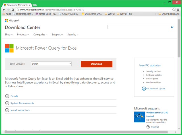
Power Query, a free add-in for Excel 2010 and Excel 2013 is easily installed. Just search for “power query download” in your search engine of choice. Or click on Figure 1.

Figure 1

It is important that you download the version that matches your version of Excel, 32-bit or 64-bit.

Figure 2

To determine which version of Office you are running, see this link.

The installation wizard will walk you through the process. The steps are clear so I will not go into it here. Once the installation is complete, there will be a new option for you in Excel.

Figure 3

Clicking this option will activate the Power Query ribbon. This is where the journey of working with Power Query begins.

Figure 4

Figure 5 shows the basic options for sourcing data. We will go into these options, and demonstrate a few, and the next post in this series.

Figure 5

Figure 6

The options in Figure 6 are used for combining queries that already exist, Merge and Append. We will cover those later in the series as well.

Figure 7

The option shown in Figure 7, Workbook Queries, is used to turn the Workbook Queries pane on or off.

Turning it on allows you see the queries that already exist in the workbook, as shown in Figure 8.

Figure 8

Once you have started a query by choosing a data source, or you have opened an existing query, you will have access to the Query Editor, as shown in Figure 9.

Figure 9

The sections of the Query Editor are as follows (corresponding to the labels in Figure 9):

1. Query Editor Toolbar/Ribbon: This is where we find the various buttons we can use for taking actions on our data. For a while, it was just called the Query Editor Toolbar. Lately, I have been seeing documentation from Microsoft referring to it as the Query Editor Ribbon. I prefer to call it the Ribbon since the similar structure in the rest of Office is called the Ribbon.

2. Formula Bar: All actions taken in the Power Query interface actually generate code using the Power Query Formula Language, known informally as M. In the Formula Bar, you can see the M code the currently selected query step. This bar is turned off by default. When you are first getting started, leaving it off is just fine. Once you feel ready to start learning more about M, then turning it on can help you with that by showing you the M code for each step you take.

3. Results Pane: This window shows you what your data looks like AFTER the execution of the currently selected query step.

4. Query Settings: This window holds a few properties of the query as a whole. The first the name of the query. I encourage you to choose an appropriate name for each query you make. Not only will it make more sense when you or someone else looks at it later, but it will also determine the name of the resulting table that gets created once you have loaded the results of the query to Excel.

This concludes this first post on the series. In the next post, we will start putting Power Query to use for importing data.